Configuration

In the following it will be explained how to add particles, add topologies, configure specifics of the selected kernel, how to record a trajectory, and how to perform checkpointing.

Adding particles

For adding particles to a system there are two separate methods. One is can be to place a single particle, one is for bulk insertion. Adding a single particle of type A to a simulation box amounts to

simulation.add_particle(type="A", position=pos)

where pos can be a list [x, y, z], tuple (x, y, z), or a numpy.ndarray: np.array([x, y, z]) with three entries representing the x,y,z components.

When one wants several particles of a certain type to the simulation, one can can exchange multiple calls to simulation.add_particle by the better performing variant

X = np.random.random((100, 3))
simulation.add_particles(type="A", positions=X)

taking a (N, 3)-shaped numpy array as position argument, resulting in N particles with their respective positions being added to the simulation. In this example, 100 particles of type A would be placed uniformly at random in $[0,1)^3$.

Adding topologies

A topology can be added by invoking

my_topology = simulation.add_topology(topology_type="My topology type", particle_types="T", 
                                      positions=np.random.random((100, 3)))

which requires a “My topology type” topology type and a topology species “T” to be registered in the ReactionDiffusionSystem. In this example the topology will contain 100 randomly placed topology particles of type “T” that are for now disconnected. If the topology should contain several different particle types one can pass a list of particle types to the particle_types argument that contains types for all the positions:

my_topology = simulation.add_topology(
    topology_type="My topology type",
    particle_types=["T1", "T2", "T3", "T2", "T1"],
    positions=np.random.random((5, 3))
)

Unless the topology consists out of only one particle, one still needs to set up the connectivity graph before running the simulation. The returned object my_topology is a topology object as the ones described in topology reactions. Edges in the graph can be introduced like

my_graph = my_topology.get_graph()
for i in range(len(graph.get_vertices())-1):
    my_graph.add_edge(i, i+1)

where the indices that go into add_edge correspond to the particle positions that were entered in add_topology.

The simulation can only be executed if the graph of each topology is connected,

• i.e., there are no independent components (between each pair of vertices there is at least one path in the graph that connects them),

and for each edge there is a bond,

• i.e., all particle type pairs that are contained in the graph have at least one entry in the topology potential configuration.

Should one of these two conditions be not fulfilled, starting the simulation will raise an error.

Kernel configuration

In case of selecting the CPU kernel with a parallelized implementation of the ReaDDy model, one can change certain aspects of its behavior:

• The number of threads to be used can be selected by

  simulation.kernel_configuration.n_threads = 4
  

• Mainly due to pairwise interactions and bimolecular reactions there is a neighbor list to reduce the time needed for evaluating these. The neighbor list imposes a spatial discretization on the simulation box into cuboids. In the default case, each of these cuboids has an edge length of at least the maximal cutoff radius / reaction radius. This means that instead of naively looping over all particle pairs ($\mathcal{O}(N^2)$), one can assign each particle to its cuboid and then loop over all particles in a cuboid and its 26 neighboring cuboids to find particle pairs.

  When collecting particle pairs in this fashion one effectively approximates a sphere with cuboids. The number of potential interaction or reaction partners can be further reduced by using only a fraction of the edge length but increasing the search radius of the neighboring boxes so that one still covers at least the cutoff radius in each spatial dimension.

  Reducing the edge length usually comes with a price, at some point the bookkeeping of neighboring boxes dominates the runtime.

  The edge length and therefore search radius can be controlled by

  simulation.kernel_configuration.cell_linked_list_radius = 4
  

  which would yield cuboids with $\frac{1}{4}$ the edge lengths of the default case.

Recording a trajectory

ReaDDy records trajectories and observable data in HDF5 files. For doing so one needs to set an output file

simulation.output_file = "my_trajectory.h5"

and instruct the simulation to record a trajectory:

simulation.record_trajectory(stride=1, name="", chunk_size=1000)

The stride arguments causes the trajectory to be recorded every stride time steps. If a name (other than the default one) is given, the trajectory data will be stored in a different data set. The chunk_size is mainly a performance parameter that has an effect on how large every chunk of data in the binary file is going to be, influencing the time needed for IO during the simulation and the resulting file size.

For reading back the trajectory data, please refer to post-processing.

NOTE: When running long simulations on a cluster it can happen that the process runs into a timeout causing the already recorded data to be corrupted. This can possibly be mitigated by configuring the job manager to send SIGINT before KILLing the process. That way the file can still be properly closed (see issue #220, thanks @jansteinkuehler). Please make sure this works in your environment before running long simulations.

Checkpointing

Checkpoints in ReaDDy consist out of the particles’ and topologies’ configurations at specific points in simulation time. They can be enabled by calling

simulation.make_checkpoints(stride=1000, output_directory="checkpoints/", max_n_saves=10)

which causes checkpoints to be made every 1000 steps. Each checkpoint is a separate file and all checkpoint files will be saved to the directory specified by output_directory. The option max_n_saves decides how many checkpoint files are allowed to be saved to the directory, e.g. if max_n_saves=10 then only the last 10 most recent checkpoints are kept.

Once the simulation has run its course and checkpoint files have been written, they can be listed by

simulation.list_checkpoint_files('checkpoints/')

A particular checkpoint file can in principle also contain multiple checkpoints. They can be inspected by

simulation.list_checkpoints('checkpoints/checkpoint_10000.h5')

and a system’s state can be restored by a call to

simulation.load_particles_from_checkpoint('checkpoints/checkpoint_10000.h5')

amounting to restoring the latest checkpoint of that particular file. If the file contains multiple checkpoints, let’s say 5, you can select the 5th checkpoint by supplying the optional argument n=4 (enumeration starts at n=0 per file).

Oftentimes you just need the last checkpoint of all checkpoint files in a certain directory. This can be achieved by

simulation.load_particles_from_latest_checkpoint('checkpoints/')

It should be noted that if the simulation should be continued and the output_directory for the new checkpoints is the same as of the original simulation, the old checkpoint files will be overwritten. If you want to keep the checkpoints of the original simulation, specify another output_directory.

Observables

The currently available observables are:

• Radial distribution function
• Particles
• Particle positions
• Number of particles
• Energy
• Forces
• Reactions
• Reaction counts
• Virial
• Pressure

There are three things that all observables have in common: The evaluation can be strided, they can have a callback function and they can be saved to the simulation.output_file.

The callback is usually a function that takes one argument being the current value of the observable. During the course of the simulation this callback function will be evaluated whenever the particular observable is evaluated.

Per default, whenever an output_file is given, the registered observables’ outputs are saved to that file. Each observable has a certain place in the group hierarchy of the HDF5 file, however this place can be modified so that, e.g., multiple observables of the same type can be recorded into the same file. To this end, the save argument of the respective observable can be modified. By providing

• None or False writing the results to file can be switched off,
• providing a dictionary with keys 'name' and 'chunk_size' can modify the name under which the observable data is stored in the group hierarchy and the hdf5 chunk size. The chunk_size is always to be considered into the “temporal direction”, i.e., if an observable yields data in the form of 3x3 matrices each time it is evaluated, a chunk would be of shape (3, 3, chunk_size).

Radial distribution function

The radial distribution function for certain particle types can be observed by

def rdf_callback(current_value):
    print(current_value)

simulation.observe.rdf(
    stride=1, 
    bin_borders=np.linspace(0., 2., 10), 
    types_count_from=["A"], 
    types_count_to=["B"], 
    particle_to_density=1./system.box_volume,
    callback=rdf_callback)

which causes the observable to be evaluated in each time step (stride=1) and print the value (callback=rdf_callback). The RDF is determined by calculating the distance from all particles of a type contained in types_count_from to all particles of a type contained in types_count_to and then binning the distance into a histogram as given by bin_borders. The histogram is normalized with respect to $g(r) = 4\pi r^2\rho dr$, where $\rho$ is the number density of particles with types contained in types_count_to, reflected by particle_to_density.

Particles

This observable records all particles in the system, as in: Each particle’s type, (unique) id, and position. It can be registered by

def particles_callback(particles):
    types, ids, positions = particles
    print("Particle 5 has type {}, id {}, and position {}."
          .format(types[5], ids[5], positions[5])

simulation.observe.particles(
    stride=5,
    callback=particles_callback,
    save=False
)

where the argument of the callback function is a 3-tuple containing a list of types, unique ids, and positions corresponding to each particle in the system. In this example the callback function prints these properties of the fifth particle every fifth time step, the output of the observable is not saved into the trajectory file (save=False).

Particle positions

The particles’ positions can be recorded by

simulation.observe.particle_positions(
    stride=200, 
    types=None, 
    callback=lambda x: print(x)
)

which makes this observable very similar to the particles one, however one can select specific types of particles that are recorded. In case of types=None, all particle positions will be recorded, in case of types=["A", "B"] only positions of particles with type A or B are returned. In this case the callback will simply print x every 200 steps, where x is a list of three-dimensional vectors. Since save is not explicitly set to False or None the observed data will be recorded into the trajectory file if n simulation.output_file was configured.

Number of particles

When one is only interested in the sheer number of particles then one can use this observable. Depending on the input, it will either observe the total number of particles or the number of particles per selected type:

simulation.observe.number_of_particles(
    stride=1,
    types=["A", "B", "C"],
    callback=lambda x: print(x),
    save=False
)

This example records the numbers of particles with types A, B, C in each time step. The callback takes a list with three elements as argument where each element corresponds to a particle type as given in types and contains the respective counts. If types=None was given, the observable would record the total number of particles, regardless of their types.

Energy

The system’s current potential energy can be observed by

simulation.observe.energy(
    stride=123,
    callback=lambda x: print("Potential energy is {}".format(x)),
    save=False
)

where stride=123 indicates that the observable will be evaluated every 123rd time step. The argument of the callback function is a scalar value and the observable’s output is not saved to a potentially configured trajectory file.

Forces

The forces acting on particles can be observed by

simulation.observe.forces(
    stride=1,
    types=["A"],
    callback=lambda x: print(sum(x))
)

yielding an observable that is evaluated every time step (stride=1) and collects the forces acting on all particles of type A. If types=None, all types are considered. The callback function takes a list of vectors as argument. Since save is not further specified, this observable would be recorded into the trajectory file.

Reactions

This observable records all occurred reactions in the system for a particular time step. It can be registered by invoking

def reactions_callback(reactions):
    for r in reactions:
        print("{} reaction {} occurred: {} -> {}, position {}"
              .format(r.type, r.reaction_label, r.educts, r.products, r.position))
    print("----")

simulation.observe.reactions(
    stride=5,
    callback=reactions_callback
)   

where stride=5 indicates that the observable is evaluated every fifth time step. The callback takes a list of reaction records as argument, where each reaction record stores information about the

• type of reaction (r.type), i.e., one of conversion, fission, fusion, enzymatic, decay,
• reaction name (r.reaction_label), i.e., the name under which the reaction was registered in the system,
• educt unique particle ids (r.educts) as in the particles observable,
• product unique particle ids (r.products),
• and position (r.position) of the reaction event which is evaluated to the midpoint between educts in case of a bimolecular reaction.

Since the save argument was left out, it is defaulted and given a simulation.output_file, the observed reactions are recorded.

Reaction counts

Instead of recording all reaction events one can also record the number of occurred reactions per registered reaction per time step. This can be achieved by

simulation.observe.reaction_counts(
    stride=2,
    callback=lambda x: print(x),
    save=False
)

where stride=2 causes the observable to be evaluated every second time step. The callback function takes a dictionary as argument where the keys are the reaction names as given in the system configuration and the values are the occurrences of the corresponding reaction in that time step.

Virial

This observable evaluates the pressure virial according to pair-wise forces by evaluating

where $\mathbf{r}_{ij}$ is the vector difference between the positions of particle i and j, $\mathbf{f}$ the pair-wise force.

It can be registered by

simulation.observe.virial(
    stride=5,
    callback=lambda x: print(x)
)

which causes it to be evaluated every fifth time step (stride=5). The callback function takes a numpy array of shape (3,3) as argument.

Pressure

The pressure of a system can be understood in terms of the trace of a pressure tensor

which is defined via the virial tensor

where $V$ is the system’s volume, $N_t$ the number of (physical) particles that somehow partake in the dynamics of the system, and $k_BT$ the thermal energy.

Observing the pressure in a simulation amounts to

simulation.observe.pressure(
    stride=1,
    physical_particles=["A", "B", "C"],
    callback=lambda p: print("current pressure: {}".format(p))
)

where stride=1 causes the pressure to be evaluated in every time step, physical_particles are set to be particles of type A, B, or C (physical_particles=None causes all particles to be considered physical), and the callback function takes a scalar value as argument.

Internally, the pressure observable builds up on the virial observable and the number_of_particles observable and when writing it to file not the actual pressure is recorded but the output of these other two observables. In the HDF5 group hierarchy the observable’s group is per default postfixed by _pressure, causing the virial to be stored under virial_pressure and the number of particles under n_particles_pressure.

Changing the postfix amounts to providing a dictionary to the save argument with

pressure_save_options = {
    'name': "empty_or_other_postfix",
    'chunk_size': 500
}
simulation.observe.pressure(1, ["A", "B", "C"], save=pressure_save_options)

where the chunk_size refers to the HDF5 chunk size of data sets.

Running the simulation

Per default, the simulation loop looks like below

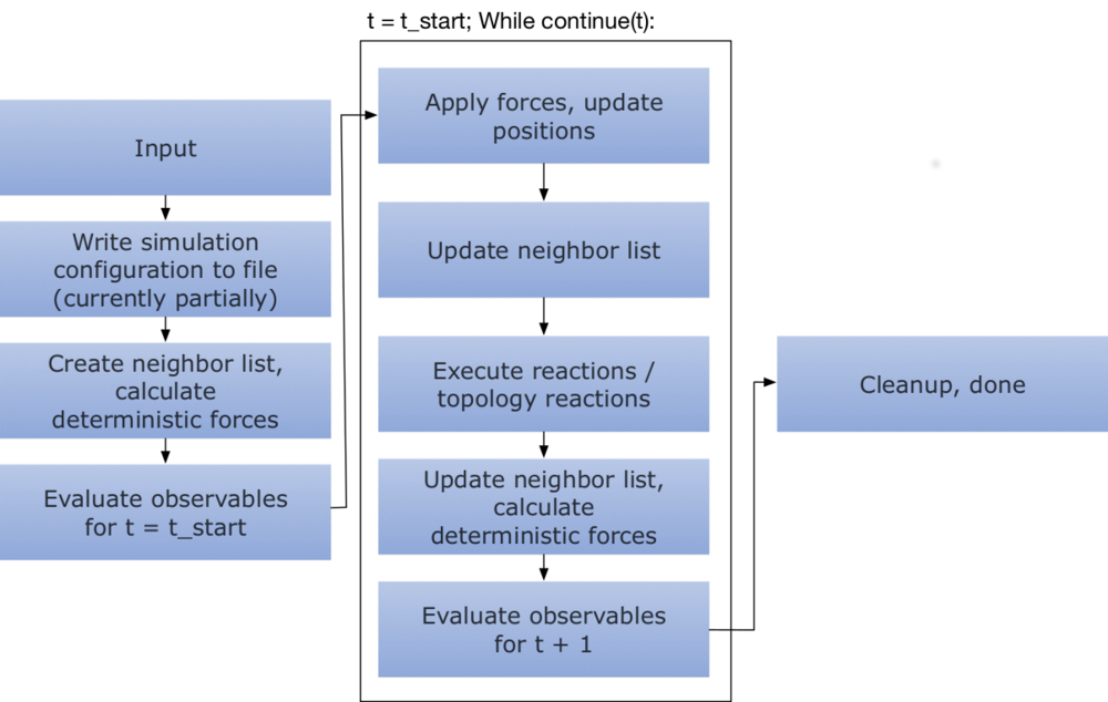
This means that all observables are evaluated at the initial state regardless of their stride, after which the actual loop is performed.

A simulation is started by invoking

simulation.run(n_steps=1000, timestep=1e-5)

where n_steps is the number of time steps to perform and the timestep is the time step. Per default an overview of the system configuration is printed upon simulation start, this can be disabled by providing the argument show_system=False.

One can influence portions of the loop through the simulation object:

• Per default a progress bar is shown when the simulation is executed, however it can be hidden

  print(simulation.show_progress)
  simulation.show_progress = False
  

• If one does not want to evaluate topology reactions at all, one can invoke

  simulation.evaluate_topology_reactions = False
  

• Evaluation of forces can be deactivated by invoking

  simulation.evaluate_forces=False
  

• Evaluation of observables can be switched off altogether by

  simulation.evaluate_observables=False
  

  Note that setting this to False also causes the trajectory to not be recorded.

• In case of a large simulation box but small interaction radii one can sometimes boost performance by artifically increasing the cuboid size of the neighbor list’s spatial discretization by setting

  simulation.skin = s
  

  where $s\geq 0$ is a scalar that will be added to the maximal cutoff.

Furthermore, one can select the

• Integrator
• Reaction handler

Integrator

Currently the only available integrator is the EulerBDIntegrator which is selected by default and can be selected by a call to

simulation.integrator = "EulerBDIntegrator"

It integrates the isotropic brownian dynamics

with an Euler-Maruyama discretization

where

Reaction handler

Reactions in ReaDDy are evaluated per time step, meaning that each particle might have multiple possible reaction partners. In order to solve this, one can chose between two different reaction handlers:

• The UncontrolledApproximation reaction handler is the less rigorous of the two. It performs as follows:
  1. A list of all possible reaction events is gathered.
  2. For each element of this list a decision is made whether it is to be evaluated based on the time step and its rate as described in the section about reactions.
  3. The filtered list is shuffled.
  4. For each event in the list evaluate it unless its educts have already been consumed by another reaction event.

  A problem of this reaction handler is that it does not give preference to reaction events based on their rate in case of a conflict, i.e., two events that share educts. However in the limit of small time steps this problem disappears.

  This reaction handler can be selected by invoking

  simulation.reaction_handler = "UncontrolledApproximation"
  

• The Gillespie reaction handler is the default choice and is statistically exact in the sense that it imposes a Gillespie reaction order on the events of a particular time step:

  A list of all possible reaction events is gathered. Then

  1. Each reaction event is assigned its normalized reaction rate $\lambda_i/\sum_i\lambda_i$
  2. A random event is picked from the list based on its normalized reaction rate, i.e., a uniform random number between 0 and 1 is drawn and then used together with the cumulative normalized reaction rates to determine the event
  3. Depending on its rate the reaction described by the event might be performed:
     • if not the event is simply removed from the list
     • if it was performed it is also removed and any other event that shared educts with this particular event
  4. if there are still events in the list go back to 1., otherwise stop

  An example of conflicting reaction events with expected outcome might be

  $$ \left\{ \begin{array}{rcc} A + B &\xrightarrow{\lambda_1}& C\\ A &\xrightarrow{\lambda_2}& D \end{array} \right. \xrightarrow{\lambda_1 \gg \lambda_2} \left\{ \begin{array}{rcc} A + B &\xrightarrow{\lambda_1}& C\\ &\mathrm{ignored} \end{array} \right. $$

  This reaction handler can be selected by invoking

    simulation.reaction_handler = "Gillespie"